Monte Carlo forecasting for software project estimation
In 1946, the mathematician Stanislaw Ulam was recovering from an illness and playing a lot of solitaire. He wanted to know the odds that a game of Canfield would come out, so he tried to work it out with combinatorics. It got ugly.
So he had a lazier idea. Lay it out a hundred times and count the wins.
That’s the whole method. Nicholas Metropolis’s own account of the early days at Los Alamos tells how John von Neumann saw what it could do once a computer did the dealing. Metropolis supplied the name, after the casino where an uncle of Ulam’s “just had to go.” Its first job was neutron diffusion in weapons physics.
It is now used to answer “when will the login page be done.” Every technique gets a retirement.
The reason it works on software is the reason it worked on solitaire. “When will we finish?” has too many moving parts to calculate and is very easy to play out.
A single estimate is one hand of solitaire
A traditional estimate plays the project once, in your head, and reports how that game went. “Twelve weeks.” It sounds precise. It’s a sample size of one.
We had one of these at CardBoard. An engineer estimated six months to refactor our tracker integrations, and the whole refactor took a year. A range wouldn’t have made the work any shorter. It would at least have put a year on the table before the year happened.
Monte Carlo analysis plays the project thousands of times, each with slightly different luck, and counts how often each finish date comes up. You get a distribution instead of a date. Most runs bunch up in the middle, and a stubborn tail finishes much later than anyone would like.
That distribution is what people mean by probabilistic forecasting. You stop saying “it will take twelve weeks” and start saying “85% of the simulated projects finished within fourteen.”
How Monte Carlo analysis works
The mechanics come in four steps, and you won’t need a math degree for any of them.
- Pick the variables that change the outcome. For software that’s usually how many stories are left, how many the team finishes per sprint, and how much new scope turns up.
- Give each variable a range or a history. That can be a guess with odds (“70% of the time a feature like this takes two weeks, 20% three, 10% four”). Better, it can be real numbers from your own team’s past sprints.
- Run the scenario thousands of times. Each run draws a random value for every variable and plays the project to the end. A spreadsheet does 10,000 runs in seconds.
- Sort the finish dates and read them as odds. The date that 85% of runs beat is your 85% forecast.
Most of the judgment lives in step 2.
Use your team’s history, not your team’s hopes
The first version of this post told you to assign probabilities to variables like code complexity and developer skill level. You can do that. Mostly you’ll be simulating your own optimism.
What holds up better is sampling from throughput, meaning how many items the team actually finished in each past sprint or week. It’s the approach Daniel Vacanti builds his book When Will It Be Done? around. You don’t estimate the team’s speed. You replay it.
Throughput already has the sick days and the surprise bugs baked in. Your guesses don’t, because nobody plans to lose a Tuesday.
A worked example, with real arithmetic
The team in this example is made up. The simulation isn’t.
It has 60 stories left. Its last eight sprints finished 6, 9, 4, 8, 7, 11, 5, and 8 stories.
The average is 7.25 a sprint, and 60 divided by 7.25 is about 8.3 sprints, which is the number most people would say out loud in a planning meeting.
Now run it as Monte Carlo. For each simulated sprint, pick one of those eight past results at random and subtract it from 60. Keep going until you hit zero and count the sprints. Then do the whole thing 10,000 times.
| Finished within | Share of 10,000 runs |
|---|---|
| 7 sprints | 6% |
| 8 sprints | 41% |
| 9 sprints | 82% |
| 10 sprints | 98% |
The eight-sprint answer from the average comes true in 41% of runs. It’s a worse bet than a coin toss, delivered with total confidence.
Nine sprints is 82% and ten is 98%. Those are the numbers I’d bring to the conversation, as a range: most likely nine, very likely by ten. If someone needs one date for a contract, give them the 85% date and tell them that’s what it is.
The spread tells you something the average hid, too. Lucky runs and unlucky runs are about three sprints apart. That’s how much variability lives in this team’s process, and it’s a more useful thing to talk about than whose estimate was wrong.
Add the scope you haven’t found yet
The example assumes the 60 stories are the 60 stories. They never are. Someone splits a story in two, and someone else remembers the admin screen.
So model the backlog as a range too. Troy Magennis’s free Multiple Feature Cut Line Forecaster spreadsheet takes a low and high guess for story count, plus a low and high guess for throughput, and runs the simulation for you. I fill it in step by step in Hate estimating? Forecast from a user story map instead.
For the high guess, take your current count and add whatever your last project grew by. If nobody wrote down what your last project grew by, start writing it down on this one.
Reading the results
Most Monte Carlo tools give you two views.
The histogram shows how many runs finished on each date. The tall bars in the middle are the likely outcomes, and the tail on the right is the risk. That right tail is almost always the longer one. Projects rarely finish shockingly early.
The likelihood table turns the same runs into odds, like 50% by this date and 85% by that one. This is the view to bring to a stakeholder.
A common habit is to plan at 85%. Below 50% you’re promising a date that fails more often than it works, and above 95% the dates get so padded that nobody believes them anyway.
What it’s good for
The obvious win is replacing a date with odds. “When will it be done?” gets an honest answer that carries its own uncertainty.
The less obvious one is risk. A wide gap between the 50% and 85% dates means the process itself is unpredictable, and that’s worth fixing before any particular deadline.
It also helps you decide what to cut. Run the forecast on the first release slice alone, then the first two, and you can see which scope line fits which date. Rerun it every sprint with the new count and the new throughput, and the forecast moves as you learn, the way a weather forecast does.
Where it breaks
Bad history makes bad dates. If the team changed size, or lost three sprints to an incident, the past isn’t a fair sample of the future. Use the recent stretch that looks like the work ahead.
Counting stories assumes they’re roughly comparable. That works when stories are split to a similar size. It stops working when one “story” is a login button and the next is billing.
It forecasts delivery, not value. A perfect forecast for the wrong scope is still the wrong scope.
Older guides warn that the simulations are slow and expensive to run. On a laptop, 10,000 runs of a backlog finish before the spreadsheet does. The expensive part is the thinking in step 2.
Where the story count comes from
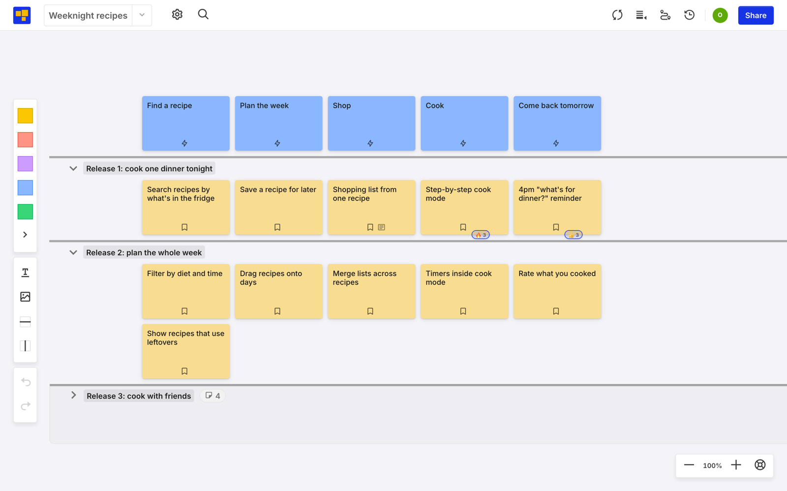
All of this needs one number to start with, the count of stories left. The easiest place I know to get it is a user story map, because the map shows the whole job and its release slices cut the job into pieces you can ship.
In CardBoard, a story map’s release slices are dividers across the map. Collapse a slice and it shows how many cards are inside, and that’s the count you feed the simulation. Cards also have an optional Size field, if your team would rather use T-shirt sizes or points.
If you’d rather question the estimate itself, and use it to find what you don’t know, that’s When will it be done? Software estimation for product managers.
Ulam reached for a hundred hands of solitaire because the math wouldn’t come out. Yours won’t either. That turns out to be fine.
Ready to try CardBoard for yourself? Create a free account, three boards, no credit card.